Geological Mapping Review: Analytical Methods with Planar Rock Layers

Earth Science Extras

by Russ Colson

Simplified map and stylized geological cross-section of the Duluth Igneous Complex, Duluth MN showing underlying folded and metamorphosed older rocks to the left (Thomson Fm), the layered series of the intrusive complex, the anorthosite series of the intrusive complex, and the overlying volcanic layers (mostly basalt) on the right. Intrusive dikes are shown conceptually.

 

Overview of Lesson

This lesson is intended as a review of mapping concepts and techniques, not as an introduction to analytical mapping of geological structures, and so some significant experience with mapping is assumed. However, a capable self-learner with experience using topographic and geological maps might be able to refer to online resourses in order to successfully work through the exercises.

Analytical mapping skills include the following (with those explored in the current lesson underlined).

• Completing a geological map based on topography and rock outcrops (including 3-point problems)
• Determining the strike and dip of a layer based on map pattern and topographic lines
• Calculating the dip angle, vertical thickness, and true thickness of rock layers (including construction and use of structural contours)
• Inference of overburden thickness and isopachytes
• Inference of subsurface unconformities and extent of subsurface layers
• Inference of subsurface fault surfaces and truncated layers
• Prediction of strike and dip based on geological fold map patterns
• Inference of subsurface cross-sections based on map views

Some analytical mapping practices include the following (again, those practices in the current lesson are underlined):

• Complete a geological map that has been started for you, based on the inferred dip in the rock layers and the topography.
• Calculate apparent dip along a selected cross-sectional line, given the true dip angle and direction.
• Draw a geological cross section, given the map view and dip directions and angles.
• Draw qualitative strike and dip symbols given a map view of a folded and plunging terrain.
• Figure out structure contours for a layer given three outcrops, and complete the geological map (surface exposure pattern) given the topography.
• Identify areas where a rock layer has been removed by erosion, and where it exists within a given distance of the surface.
• Given topography and exposure at the surface, figure out the dip of a fault, which side is up, and whether the fault is normal (extensional) or reverse (compressional).
• Given topography and exposure at the surface, complete the cross-sectional view of a faulted terrain, with cross-sections going in any direction.

 

Introduction to simple horizontal and tilted layers

Even if a geologist has not measured the strike and dip of a rock layer in the field (such as might be done by using a Brunton compass on the outcrop), it is possible to infer the orientation of a planar feature (such as the contact between two planar rock layers) by the relationship between the map pattern of the contact and topographic lines. For example, if a planar feature is horizontal, it must be parallel to topographic contour lines since the contour lines, representing points of equal elevation, always represent horizontal planes. In contrast, vertical planar features, such as the contact between vertical rock layers, will be completely independent of the topographic contour lines, cutting across them without regard to their direction or orientation. A tilted planar surface will lie somewhere between these two extremes.

Likewise, it is possible to infer the thickness of rock layers by comparing the contacts at the top and bottom of a rock layer with the elevations at which those contacts occur. For example, if rock layers are horizontal, it is a simple matter to observe the elevation at the top of the layer and the elevation at the bottom of the layer, and then infer the thickness to be the difference between those two elevations. If a rock is tilted, then a bit of goemetrical reasoning and calculation can still reveal the thickness based the dip of the layer and the elevations at which the top and bottom appear in the field (or on a map).

From inferences such as these, the orientation and placements of rocks underground can be reconstructed from what is seen at the surface (the map view), and illustrated in a cross-sectional view.

The exercises below work through some of these mathematical and geometric inferences for the case of tilted or horizontal planar rock layers.

Map Puzzle 1:

Although the geological map below is partially filled in with units K, L, M, and N, the map is not completed--for example, there are no rocks shown to the right of the arrow at the top of the map. Print out the partially-completed map, label all topographic contour lines, and complete the geological map showing how the geological units occur at the surface. Once you have completed your map, then attempt the exercises below (You can, of course, simply skip to doing the problems below, but without first engaging in an effort to figure out the map, the 'learning benefit' of the exercise will be strongly decreased.) 

 

 

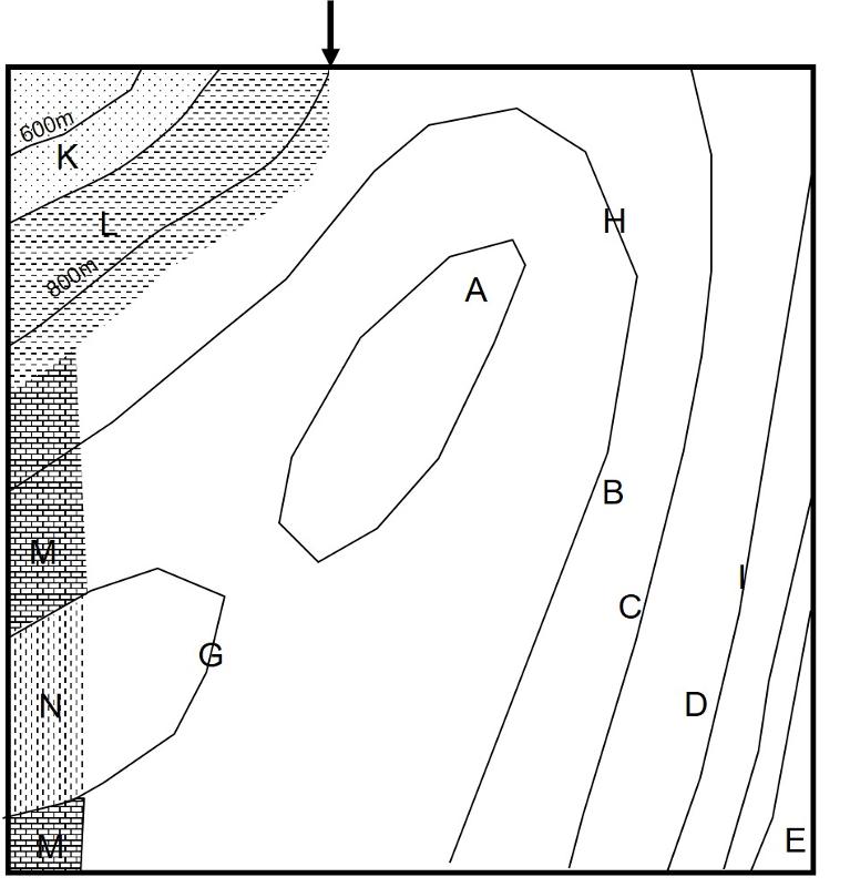
For convenience, the map is being reproduced again below.

Consider the line A-B shown in the map below. Construct a topographic profile for this line using standard methods (usually involving marking where topographic lines cross the profile line and transferring those to marks on a scaled topographic profile--search online for 'how to construct a topographic profile' if you don't know how to do this). Be sure that you have clearly labeled the vertical scale elevations. Once the topographic profile is completed, draw in the rock layers with their correct elevations, thicknesses, and slope, making sure that the contact the rock layer makes with the topographic profile line--the surface of the earth--matches where the rocks appear on the map.

 

Map Puzzle 2:

The structure contour is a powerful tool in analytical map interpretation. It is from the structure contours that we can infer strike and dip of rock layers based on map patterns, calculate dip angles and rock thickness, measure overburden depth,and infer the extent of subsurface truncating features such as faults and unconformities. Structure contours are similar to topographic contours in that they map elevation changes. However, whereas topographic contours map the elevation of the surface of the ground, structure contours map the elevation of specific structural surfaces, such as fault surfaces, unconformities, and the contact between rock layers. In the exercises for Map Puzzle 2, we will be dealing with planar (not folded) contacts between rock layers. If you are not familiar with structure contours and their use, some searching online and reading can help get you ready for the following exercises.

The basic concept for inferring structure contours from a geological map is the following: Where a structural surface encounters the surface of the earth, the elevation of the structural surface must equal the elevation of the surface topography. Thus, where a contact between rock layers shows up on a geological map, the structure contour for that contact surface at that location must equal the elevation of the topography. Where a structure contour for that contact surface is higher than the topography, that contact and the rock layers associated with it no longer exist, having been eroded away. Where a structure contour for that contact surface is lower than the topography, that surface and the rock layers associated with it are below ground beneath some depth of overburden.

To review how we construct structural contours from geological map patterns, let's consider a simple conical hill.

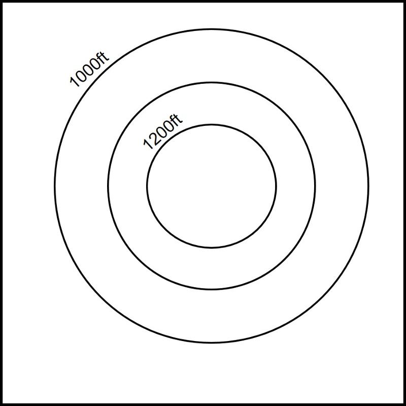
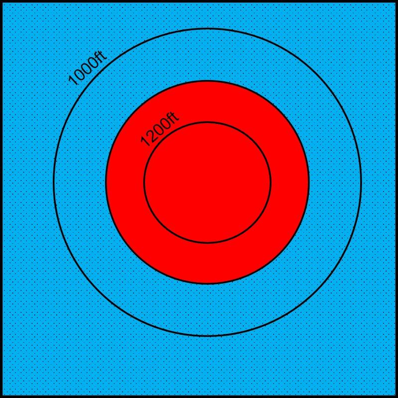
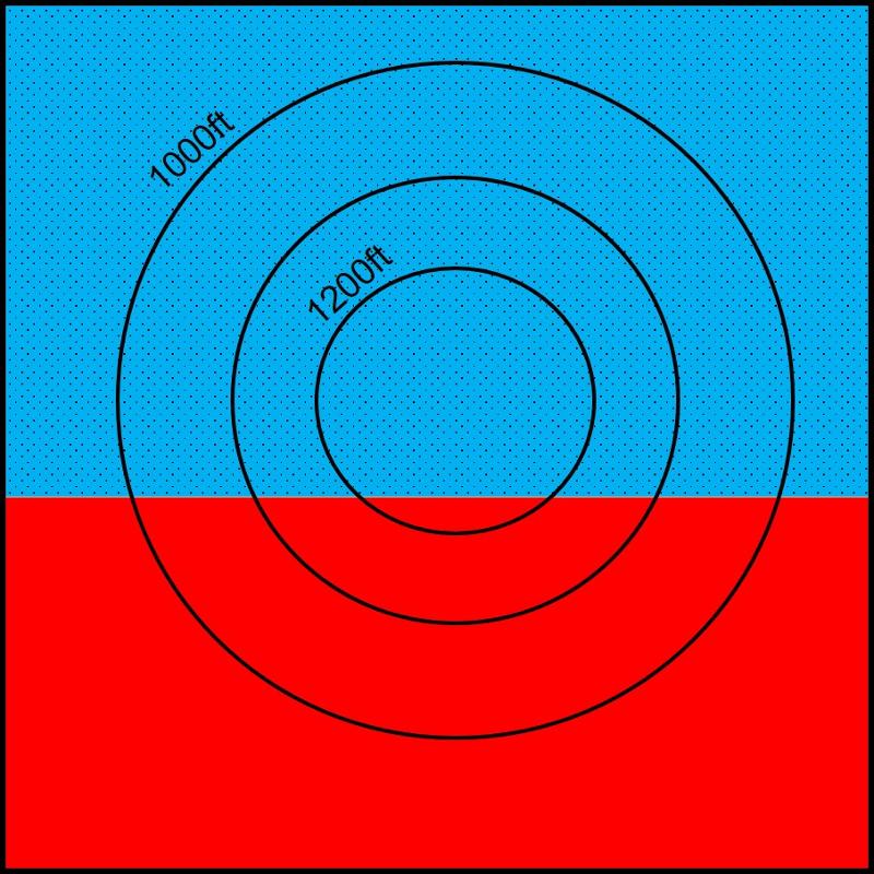
If the rock layers are horizontal, such as in the exercises for Map 1 above, then the contact between the layers (the surface that we are going to plot structural contours for) will always be at the same elevation, so there is only a single structural contour possible. For example, two horizontal layers are shown below, a red layer and a blue layer, with a contact that is always at 1100 ft regardless of location. Notice that the contact between the red and blue rocks is parallel to the topographic lines, as we mentioned was the case for horizontal rocks in the Map 1 exercises above. (blue rocks are stippled)

If the rock layers are vertical, then the surface between those layers will change elevation, but all of the different elevations will be stacked on top of each other so that, again, there is only one structure contour line. In the map below, we are considering that the red and blue layers are each sufficiently thick to fill in the entire map area. Notice that the contact between the two layers cuts across the contour lines without being influenced by topography, as we mentioned was the case for vertical rocks in the Map 1 exercises above. (blue rocks are stippled)

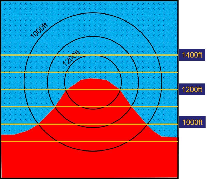
In the typical, and more interesting, case, rock layers are neither horizontal nor vertical, but dipping at some angle into the earth. This results in a case in which the contact surface between the layers is neither parallel to the topographic lines, nor independent of them, as shown below. (blue rocks are stippled). Recognize that this is a map view with the hill rising up out of the paper toward us. The red rocks are exposed at the surface in the area fanning out toward the south.

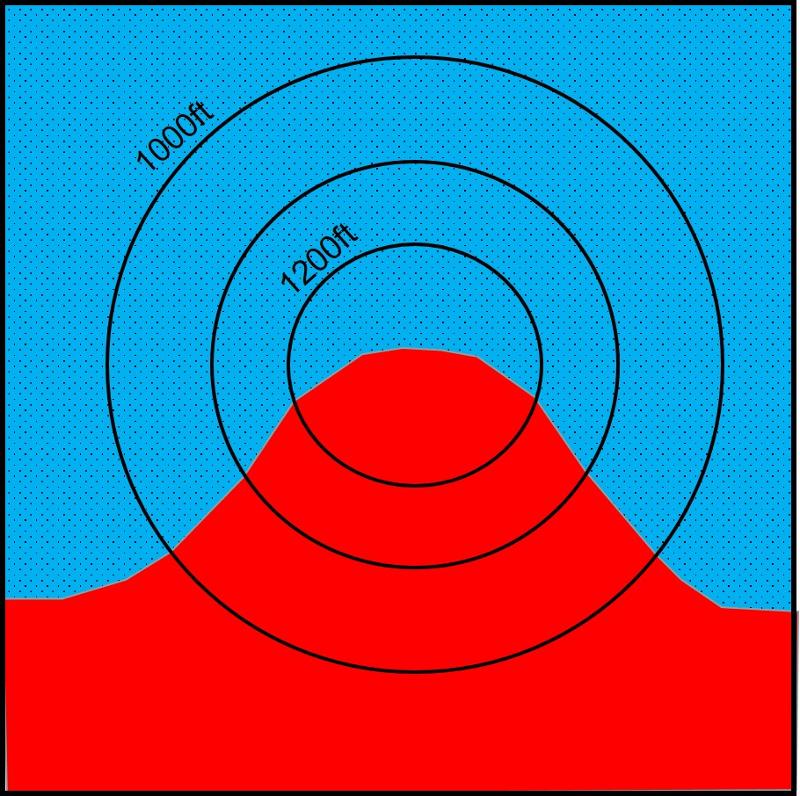
Present in the map above is information that can reveal the strike of the rock layers, the direction and angle the rocks are dipping, and which rock is on top and which is underneath.

To construct our first structural contour, consider the points at which the contact between the red and blue (stippled) layers cross the 1200ft topographic contour lines, shown by yellow stars below.

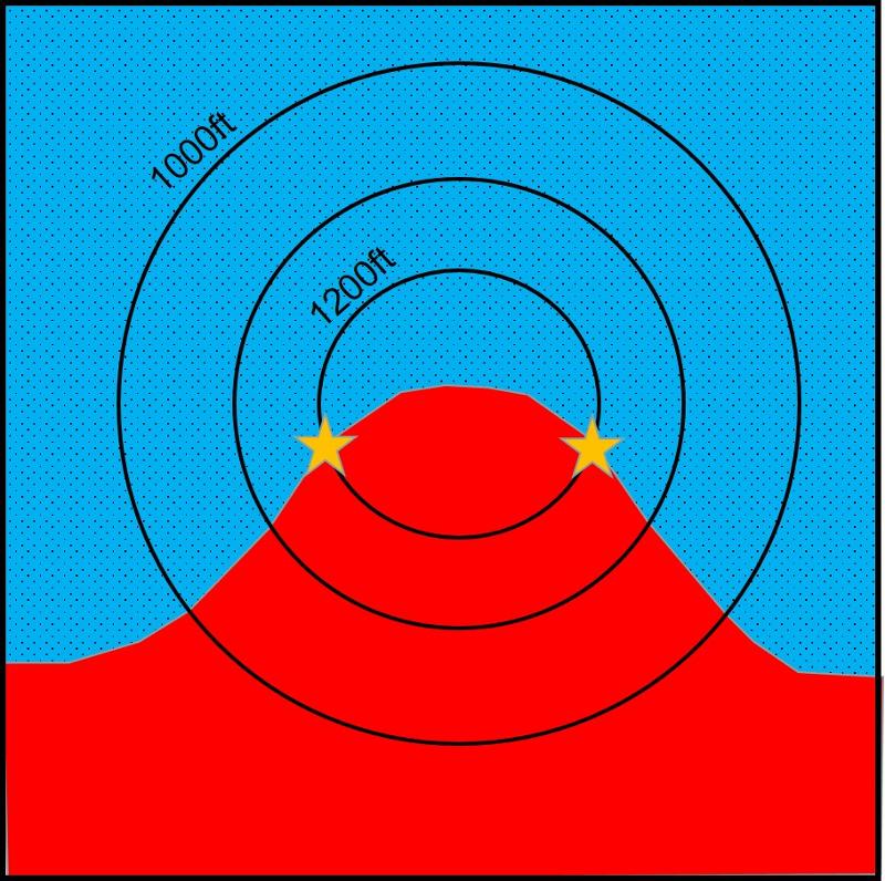
Since these points are places where the contact between the layers intersect the surface of the earth, and the elevations of the surface at those two points are both at 1200 ft, we can infer that these are two points on the 1200 ft structure contour for the contact between the layers. If the contact between the two layers is planar, then the structure contour will be linear on the map, with the line passing through these two points, as shown below.

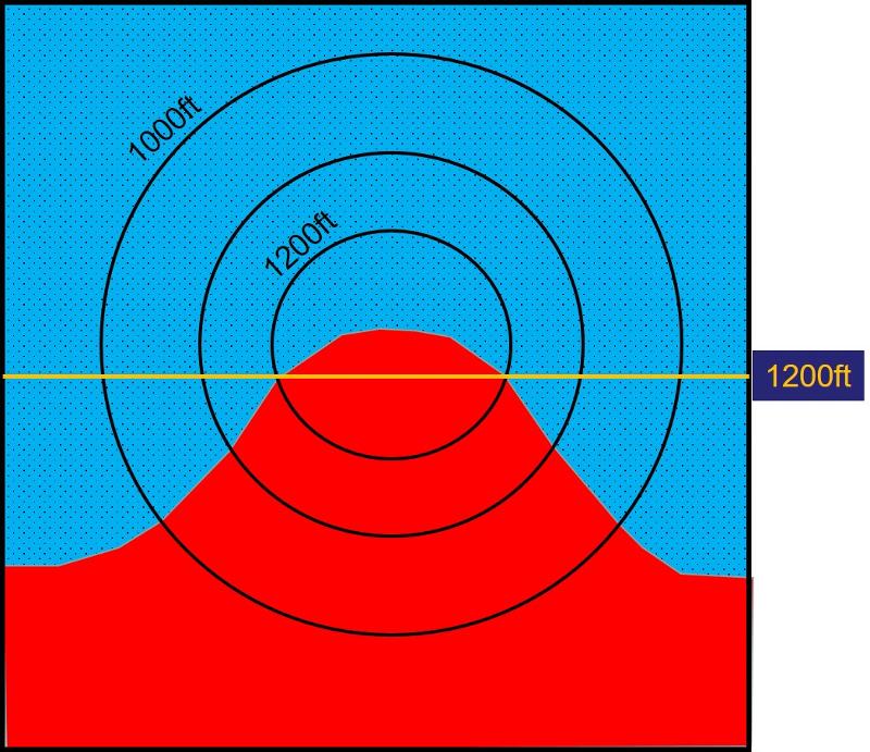
Anywhere along this line, the contact between the two planar layers (red and blue, stippled) will be at 1200 ft. Inside the 1200ft topographic contour line, the topographic elevation is higher than 1200 ft, meaning that the contact is hidden from us along the 1200ft structure contour because it is underground, and so we see only the red layer. Outside the 1200ft topographic contour line, and along the 1200 ft structure contour, the contact is higher than the elevation of the earth's surface, meaning that the contact (and the red layer) has been eroded away in these areas and no longer exists, and so we see only the blue (stippled) layer. From this alone, we can infer that the red layer is the layer on top, and the blue, stippled, layer is the layer on the bottom. We can also infer the strike to the rocks because structure contour will be parallel to the strike. Notice that the strike of the rocks is not the same as the trend of the contact between the rock layers as seen in the map! This is because the map trend of the rocks depends both on the strike of the rocks (or on the dip, which is always perpendicular to the strike) and on the way the rocks have been eroded in making the topography.

Side note: we can construct a structure contour from only two points for the case of a planar feature because two points define a line, but we would need more than two points to construct structure contours for non-planar surfaces.

In the map above, we completed a structure contour for 1200ft by drawing a line through the two points where the contact between layers intersects the 1200ft topographic contour line. We can go through a similar process to determine the 1100 foot structure contour, and the 1000 ft structure contour, as shown on the map below. If the contact is a planar surface (not curved or folded), then the slope of the contact (and the slope of the associated rock layers) will be constant and therefore the spacing of the structure contours will be constant. From this constant spacing, we can extrapolate the structure contours into regions where we don't have map data to directly reveal the elevation of the contact, as shown below for the elevations 900ft, 1300ft, and 1400 ft.

These structure contour lines portray a planar surface (the contact between the red and blue stippled layers) that is descending toward the south. The straight structure contour lines and their even spacing are consistent with a planar feature, not a folded or curving one. The structure contour at 1400ft is higher than any topographic feature in the map area, meaning that the contact in that area is projected to be 'up in the sky' meaning that it has eroded away. The 900ft structure contour is lower than any topographic feature in the map area, meaning that the contact is projected to be below ground in that area.

Make sure that you understand the methodolgy for constructing a structural contour map before proceeding to the exercises below.

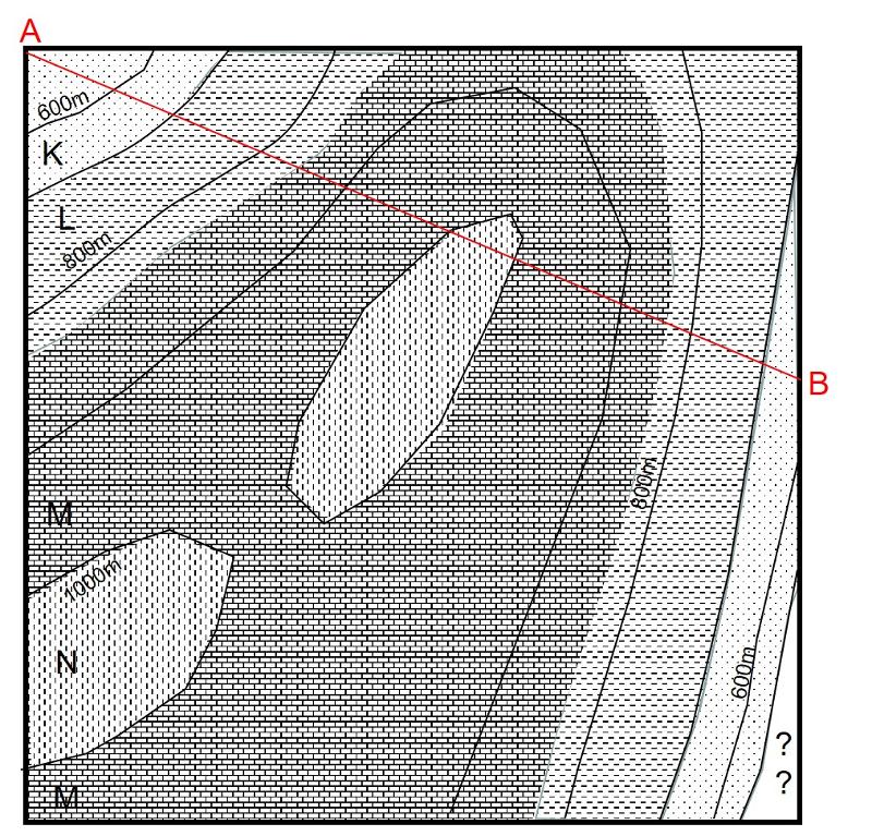
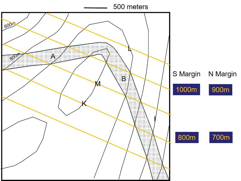
MAP 2: Consider the map for our second set of analytical mapping problems below. A single planar layer of rock is shown by the stippled area of the map. Print this map out and construct structure contours for the south boundary of the stipled rock layer. Notice that this map has the same topography as our Map 1 above, but the geology is quite different.

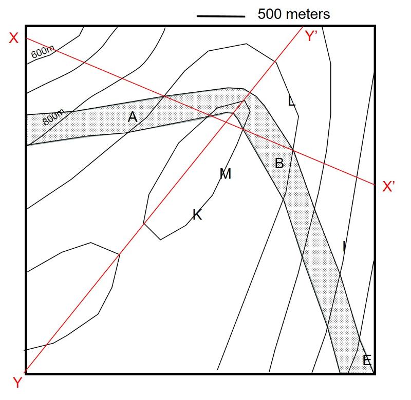
Dip angle can be inferred from these structure contour lines as well as dip direction. SInce the contact feature is planar (or nearly so) the dip angle will be the same everywhere. Like any slope, dip angle is calculated from "rise/run," the change in elevation divided by the map distance over which that change occurs. The true dip angle of the feature is the steepest dip, that is, the dip perpendicular to the strike. The change in elevation can be determined simply from the elevations of the structure contour lines. The map distance can be determined by using a ruler and the scale of the map.

The slope is then determined from the relationship

Tan ϴ = Difference in elevation/Map distance

Or ϴ = dip angle = tan^-1(Difference in elevation/Map distance)

So, for example, suppose that two structure contour lines have a difference in elevation of 200 feet. Suppose that those two structure contour lines are 2000 feet apart (map distance, using a map scale and measuring perpendicular to the strike of the rock layers. The slope will be

Or ϴ = = tan^-1(200/2000) = tan^-1(0.1) = 5.71 degrees

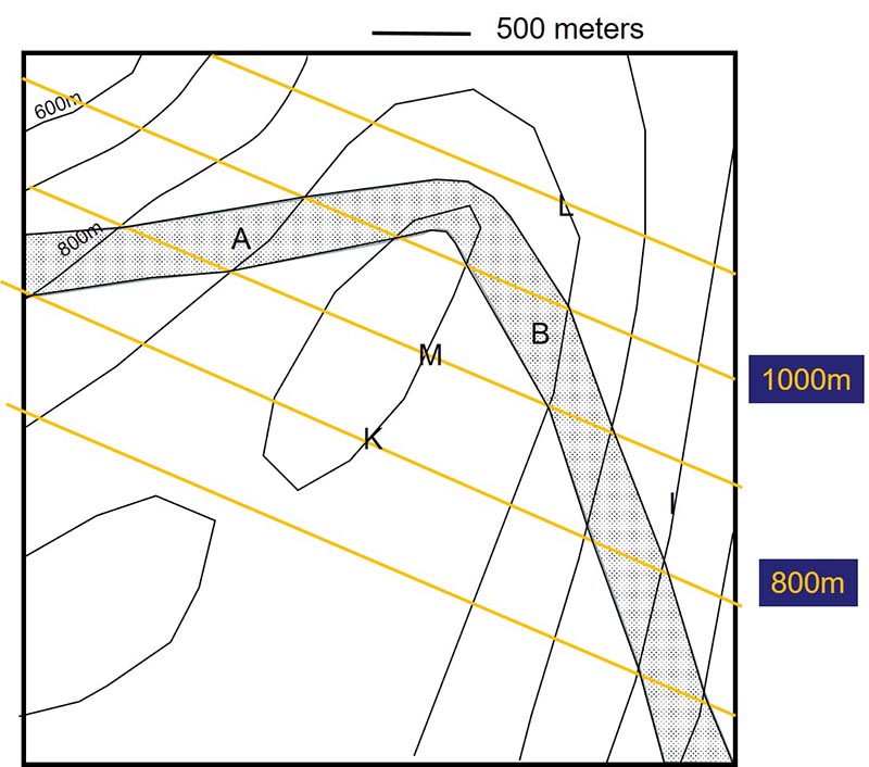
Given the trigonometric relationship above, and using your constructed structure contours, determine the slope of the contact exposed along the south margin of the stippled rock (a version of the map with structure contours is provided here for you).

We have been considering the south margin of the stippled rock layer. Take a moment to do some spatial thinking and visualize, based on the location of the margin and the direction of dip of the rock layer, whether that margin represents the top or bottom of the stipled layer. Which do you think?

You can check your conclusion by considering the structure contours for the northern margine of the stippled rock (remember, we looked at the southern margin in mapping our first set of structure contours). Because this map has been simplified and stylized, the structure contours for this surface will fall exactly on top of those for the south margin, although they will be at a different elevations (in real geological landscapes, structure contours for the top and bottom of a rock layer won't generally fall on top of each other).

Take your original structure contour map, and write on it the new structure contours for the northern margin. Which is at a higher elevation, the structure contours for the northern or southern margin? Which margin, then, is the 'top' of the stipled layer?

The structure contours for the top and bottom of the rock layer also give us a way to determine the vertical thickness of the layer. Consider the map illustration below showing the structure contours for the top (dashed lines) and bottom (solid lines) of a rock layer. The vertical thickness (that is, the vertical distance between the top and bottom of the layer), can be figured out from these structure contours. Take a minute to try to do it for the location indicated by the yellow star before reading further below.

The elevation of the bottom of the layer at the star is immediately evident from the structure contour and equals 700ft. The elevation of the top of the layer at this same spot can be figured out by interpolating between the two adjacent structure contours--it is about half way between 900ft and 1000ft, or 950 ft. Therefore, the vertical thickness is 250ft.

So what is the vertical thickness of the stippled layer in the Map 2 problem? The map is reproduced below. Although problems like this can be solved for any real rock layer, the inference in the case of this stylized map is particularly easy because the two different structure contours fall directly on top of each other, making the calculation simple.

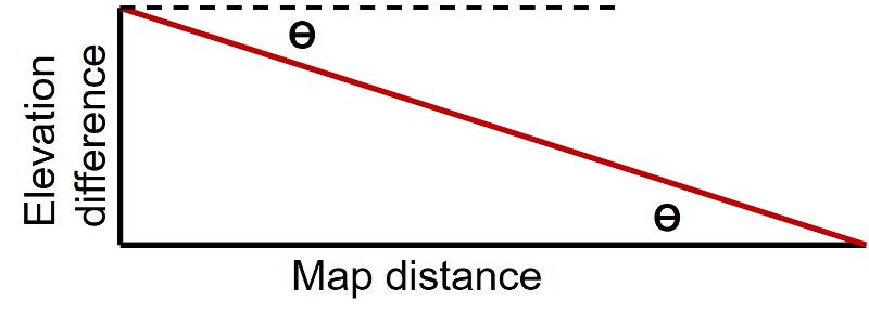
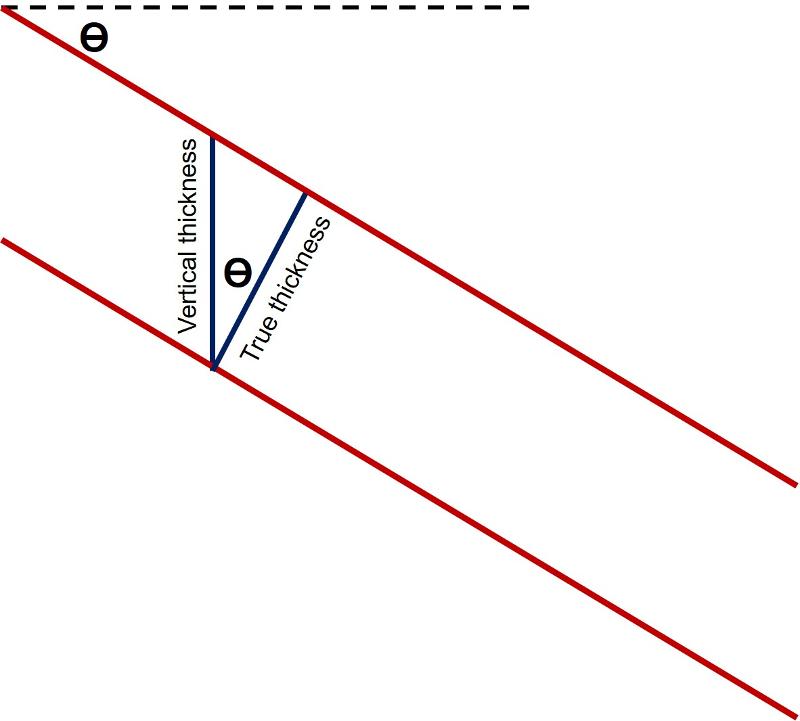
True thickness can be related to vertical thickness with a bit of trigonometry and the dip angle of the stippled layer which we determined above. Consider the cross-sectional illustration below in which ϴ is the dip angle (which has the same value as the angle between the vertical thickness line and the true thickness line). From this geometry, we see that the following trigonometric relationship will be true:

Cos ϴ = True thickness/Vertical thickness or

True thickness = Vertical thickness * Cos ϴ

Another primary use of structure contours is to allow for more precise construction of geological cross-sections. Just like topographic lines can be transferred from a map to a topographic profile by marking points along a profile line, structure contours can be transferred to a geological cross-section in the same way, charting the elevations of contact lines my marking where a section lines crosses a structural contour, allowing even contacts well below the surface to be tranferred to the cross-sectional view.

However, it's also important to be able to look at structure contours and quickly infer the approximate cross-sectional view even without the more detailed and precise contruction of a geological cross-section. This more qualitative skill is the one we will practice in the next couple of exercises.

 

Map Puzzle 3:

Introduction to Three Point Problems

Mathematically, three points define a plane. Thus, if a map surface such as a fault surface or a contact between rock layers is planar, that is, not curved, the orientation of the surface can be figured out from three outcrops, defining three points on the plane (as long as no more than two of those points are in a single line). This means that the strike and dip of the surface can be calculated, map view of the surface can be constructed, and overburden thicknesses determined based on those three outcrops of the rock.

Construction of Structure Contours:

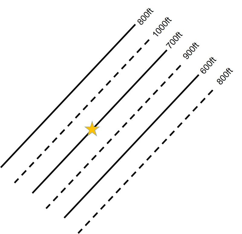
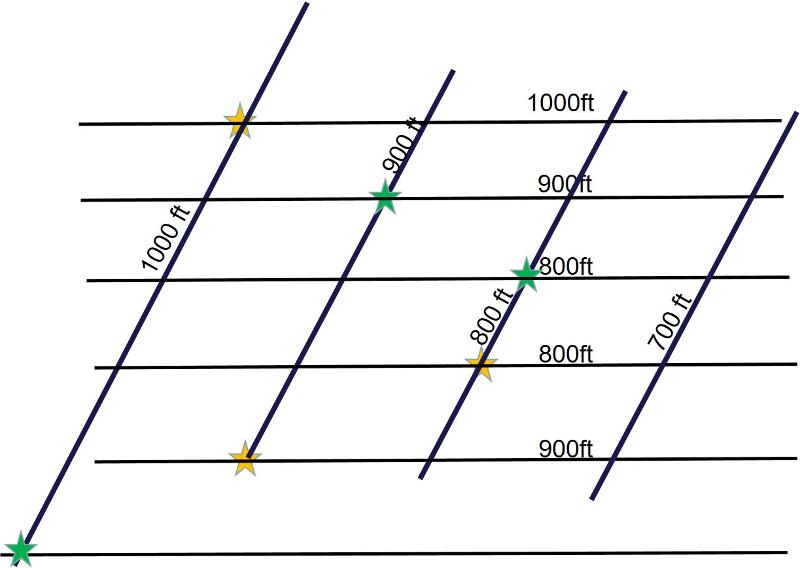
Consider the simple topographic map below showing three outcrops of a very thin planar rock layer (or a contact between two rock layers, or a fault surface), shown as yellow stars. How can you construct a structure contour line for this thin rock layer?

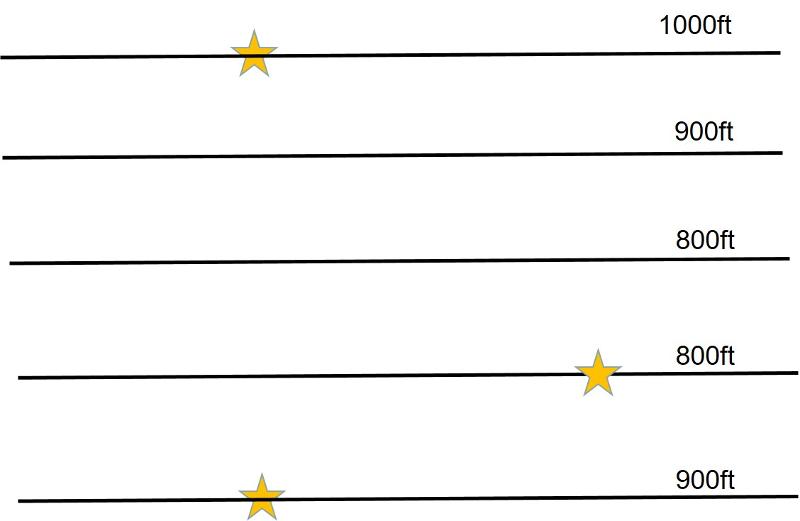
As we learned in our previous exercises, to construct a structure contour of a planar surface, we need two points that have the same structural elevation--the structure contour line passes through these two points. However, in the map above, we have a point at 1000 ft, one at 900 ft, and one at 800 ft. How do we get two points at the same elevaton so as to construct a structure contour?

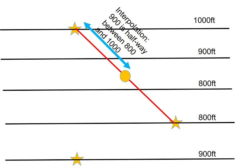
If the surface is planar, then the slope between any two points will be constant and we can interpolate the location of an intermediate elevation for the plane (If you don't know what interpolation means, you might read up on it online--it is also a critical mathematical process in constructing a topographic map from elevation data and we will use it in constructing map patterns in lessons below). In the map above, interpolation can give us a second point with a structural elevation of 900 ft. For example, the plane must be at 900 ft exactly halfway between the outcrops at 800ft and 1000 ft, as shown in the map below. Notice that the point where the elevation of the rock layer or contact reaches 900ft does not correspond to the topographic elevation of the landscape which can be seen to be close to 850 ft.

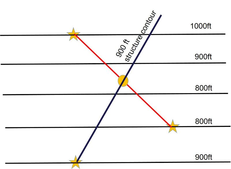
We now have the location of two points on the plane both at an elevation of 900ft, so we can draw a structure contour as we did in Map 2 above, getting the following

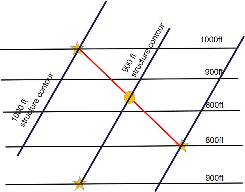
Since we are dealing with a planar feature, not a curved or folded one, the structure contours for other elevations must be parallel to this structure contour. We can therefore draw parallel structure contours through the other two points that we know, one at 800 ft and one at 1000 ft) (be aware that for 'real' maps, the outcrops don't have to fall politely on even contour lines as they do in this illustration--to solve for those real-world situations, we could simply do a bit more interpolation or extrapolation to get to even elevation numbers).

 

Construction of Map Pattern:

Once we have the structure contours, we can easily complete the geological map of the feature. The first step to do this is to predict more locations where the thin rock layer (or contact) should be found at the surface of the earth. This is simply a matter of taking note of every locaton where the elevation of the structure contour and the elevation of the landscape (topography) are the same! That is, the rock is exactly at the surface at those locations. This is shown with the green stars below. Notice that we have added another structure contour at 700 ft in order to provide us with a 'bigger' view. Although there are no known outcrops for this elevation, we can predict the location of the structure contour because, for a planar feature, the structure contours must be evenly spaced. Also, another 1000ft topographic contour line has been added to the bottom side of the map, again to give us a 'bigger view' for the purpose of this illustration.

 

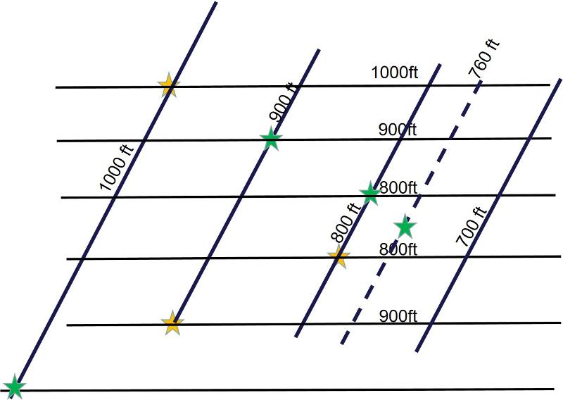
Already we can begin to see where the map pattern of this thin rock layer must go, moving from the northwest toward the southeast, and then turning from the norttheast toward the southwest. However, exactly where does this 'turning' happen? To visualize that, we need to think about what is happening between the 800ft and 700ft structure contour lines. Along the 700 ft structure contour, the rock layer will be at 700 ft. Since there are no landscape elevations as low as 700 ft, there won't be any outcrops along the 700 ft structure contour. Somewhere between the outcrops along the 800ft structure contour (marked by stars) and the 700 ft structure contour, the points where the rock reaches the surface must reach their eastern-most extent.

Notice that there is a valley in this area where the outcrop pattern 'turns.' This valley is less than 800ft in elevation, but it must be more than 700 ft in elevation, otherwise we would have another topographic contour line there. If we consider the slope of the valley wall, we can see that if the slope stayed constant, the middle of the valley would be at 750 ft. But, of course, the steepness is likely to decrease as we approach the bottom of the valley (making a "U" shape rather than a perfectly-pointed "V"). Let's approximate that the elevation of the valley at its lowest point is about 760 feet. Then the outcrop of the rock at this lowest point will be where the structure contour is 760 feet. This will occur 40% of the way from the 800ft structure contour to the 700ft structure contour. This gives us a way to interpolate another important point in our outcrop pattern, as shown below.

Now we can 'connect the dots' in a geoloically logical fashion in order to construct the map view of the thin rock layer (or contact, or fault surface). This is shown below.

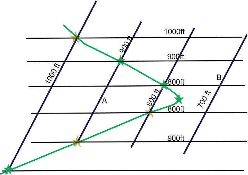
Let's take a moment to interpret this result. Ask yourself, where will the thin rock layer exist beneath the surface (with an overburden) and where will it not (where it's been eroded away)? At point A, for example, the elevation of the rock layer is 900ft while the topographic elevation is about 760 feet, so this is a spot where the rock layer has been eroded away. This will be true everywhere inside the sideways "V" defined by the outcrop. In contrast, the elevation of the rock at point B is 700ft, which is well below the topographic elevation of about 825 feet, so the rock at this locaiton still exists underground. This will be true for all locations outside the sideways "V" defined by the outcrop.

Application of three-point analysis to Map 3: Practice in map construction

For convenience, we are again using the same topography as for Maps 1 and 2, but the geology will again be different. Imagine that the stars in the map below mark the location of a thin coal seam (thin enough so that its entire thickness can be portrayed by the thickness of your map line). Print out this map and construct structure contours for the feature and then construct the map pattern based on your structure contours, in the fashion shown in the example above. The letters on this map will be used to test how good a job you did with your construction.

 

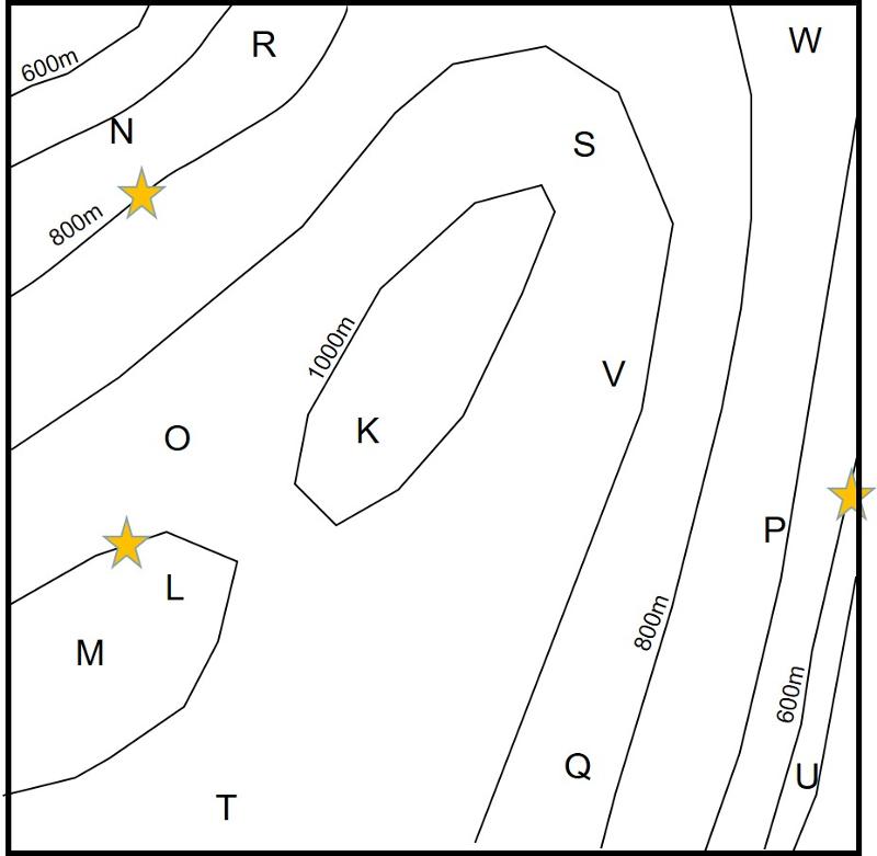
If you have done your map correctly and carefully, you should be able to correctly answer the following question. Don't be sloppy or try to answer this question too fast. There will be no partial credit for this question.

 

Map 3 and Isopachytes:

Isopachyte comes from "iso" meaning same and "pachyte" meaning thickness-and so means "same thickness." The prefix "pachy" shows up in other places too, such as in pachyderm (elephant), which means thick skin and Pachycephalosaurus which means thick head saurus!

An isopachyte line is a line showing equal thickness of something. In our case, for the exercise below, it will mean equal thickness of overlying rock.

Suppose that you wanted to evaluate the economic value of the coal seam, and to do that you need to know how much overburden material would need to be removed to get to it. You determine that it can be extracted at a profit if the depth is no more than 100 meters. In order to figure out where on the map the coal exists at 100 meters or less beneath the surface, you decide to plot an isopachyte line representing all points where the coal seam is exactly 100 meters below the surface. Then, everywhere between this line and the line that shows where the coal is exposed at the surface will have less than 100 meters overburden.

To plot the isopachyte on your map, you can do the same thing as you did to plot the map of the coal seam, except consider the points 100 meters higher than the coal seam. So, for example, where the coal seam is 900 meters, the isopachyte line will be 1000 meters, and so on. Another way to think about this is to consider each structure contour to be 100 meters higher than the coal seam, and then plot the points where the structure elevation equals the topographic elevation, just like we did to map the coal seam.

 

Practice in Spatial Thinking:

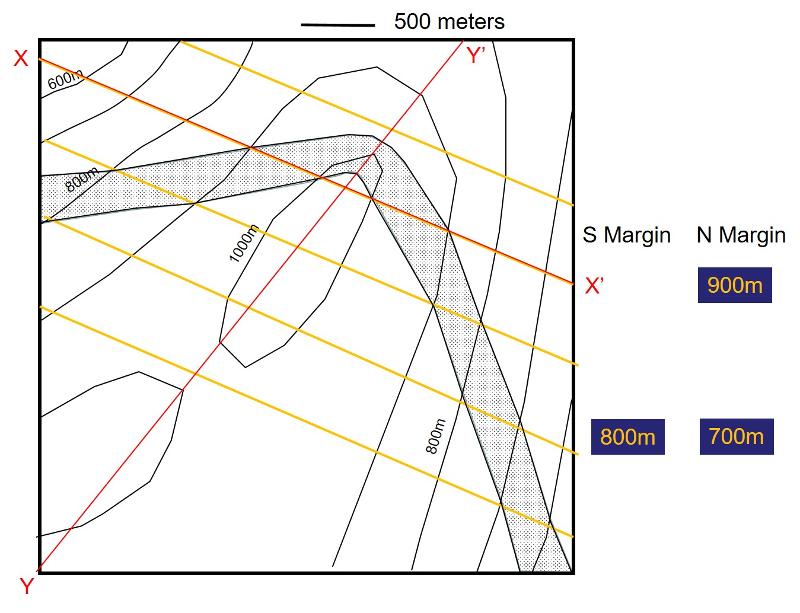
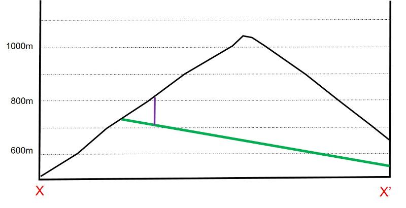
We aren't going to formally construct a geological cross-section this time, but take a few moments to consider what the cross-sections X-X' and Y-Y' would look like, given the map below (Green is the map pattern for the coal seam, purple is the isopachyte line, where the coal seam is 100m deep). Feel free to sketch out your thoughts. My solutions are given further below.

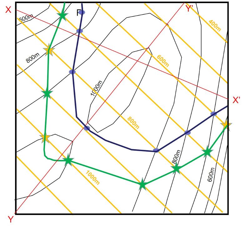
After thinking about the cross-sectional views and sketching them out, check out my solutions below. The green line is the coal seam. The purple vertical line marks the point where the coal seam is 100 meters below the surface and corresponds to the location of the isopachyte line on the map.

 

last updated 2/13/2022.   Text and pictures are the property of Russ Colson.